Phantom Validation: Bridging Simulation and Measurement
1. Introduction
Tissue-equivalent optical phantoms serve as critical tools for validating the accuracy of optical simulation models. This study employs the Phantom F04 from QUELimaging as our validation standard. With well-characterized optical parameters and reference measurement data, this phantom provides a reliable benchmark for establishing a bidirectional verification framework between simulation and measurement.
1.1 Research Objectives
This study aims to construct a comprehensive validation pipeline that verifies simulation model accuracy through the following approaches:
- Factory Data Internal Consistency Verification: Validate the consistency between factory-provided Reflectance/Transmittance ($R$/$T$) data and optical parameters ($\mu_a$, $\mu_s’$, $g$, $n$)
- Forward Simulation Accuracy Verification: Employ MOP-MCML and Adding-Doubling (AD) forward simulation tools to calculate $R$/$T$ from optical parameters and verify simulation accuracy
- Experimental Measurement and Correction: Measure actual $R$/$T$ through a dual integrating sphere system and establish correction functions mapping measurement data to factory standards
- Closed-Loop Validation: Perform inverse and forward simulations on corrected measurement data to form a complete verification loop
1.2 Phantom Specifications
Phantom F04 provides the following information:
- Optical Parameters: Absorption coefficient $\mu_a$, reduced scattering coefficient $\mu_s’$, anisotropy factor $g=0.85$, refractive index $n=1.48$
- Measurement Data: Reflectance $R$ and Transmittance $T$ for three thicknesses (3mm, 4mm, 5mm) across the 450–1500 nm band (5 nm intervals)
2. Factory Data Internal Consistency Verification
2.1 Verification Strategy
Factory data consistency verification serves as the starting point of the entire validation pipeline. Using the Inverse Adding-Doubling (IAD) algorithm, we invert optical parameters from factory-provided $R$/$T$ data and compare them against factory-specified optical parameters.
2.1.1 IAD Inversion
We employed the IAD program (version 3-16-3) to invert optical parameters from factory-provided $R$/$T$ data:
1 | ./iad -v |
For three thicknesses ($d$ = 3, 4, 5 mm), we obtained corresponding $\mu_a$ and $\mu_s’$ through inversion. Theoretically, since optical parameters are intrinsic material properties, different thickness samples should yield consistent optical parameters.
2.1.2 Forward Simulation Verification
Using factory-provided optical parameters, we performed forward simulations via MOP-MCML and AD to calculate $R$/$T$ for different thicknesses:
MOP-MCML Configuration:
1 | clang -std=c11 -O3 -ffast-math -mcpu=native -flto \ |
For MOP-MCML usage, refer to the MOP-MCML: A User Guide and Technical Introduction. For AD usage, refer to Introduction to Inverse Adding-Doubling (IAD).
2.2 Validation Metrics
To quantify the discrepancy between simulation and reference data, we define the relative error as:
$$
D = \left| \frac{X_{\text{simu}} - X_{\text{ref}}}{X_{\text{ref}}} \right| \times 100%
$$
where $X$ can represent Reflectance $R$, Transmittance $T$, or optical parameters $\mu_a$, $\mu_s’$.
2.3 Results Analysis
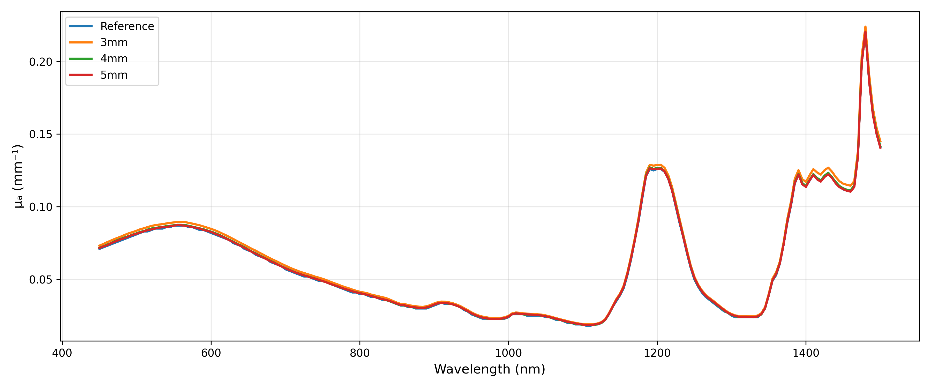
The IAD inversion results demonstrate that optical parameters retrieved from three different thickness samples are fundamentally consistent, aligning with the theoretical expectation that optical parameters are intrinsic material properties. The deviation between inverted parameters and factory-provided parameters falls within reasonable bounds, proving the internal consistency of factory data.
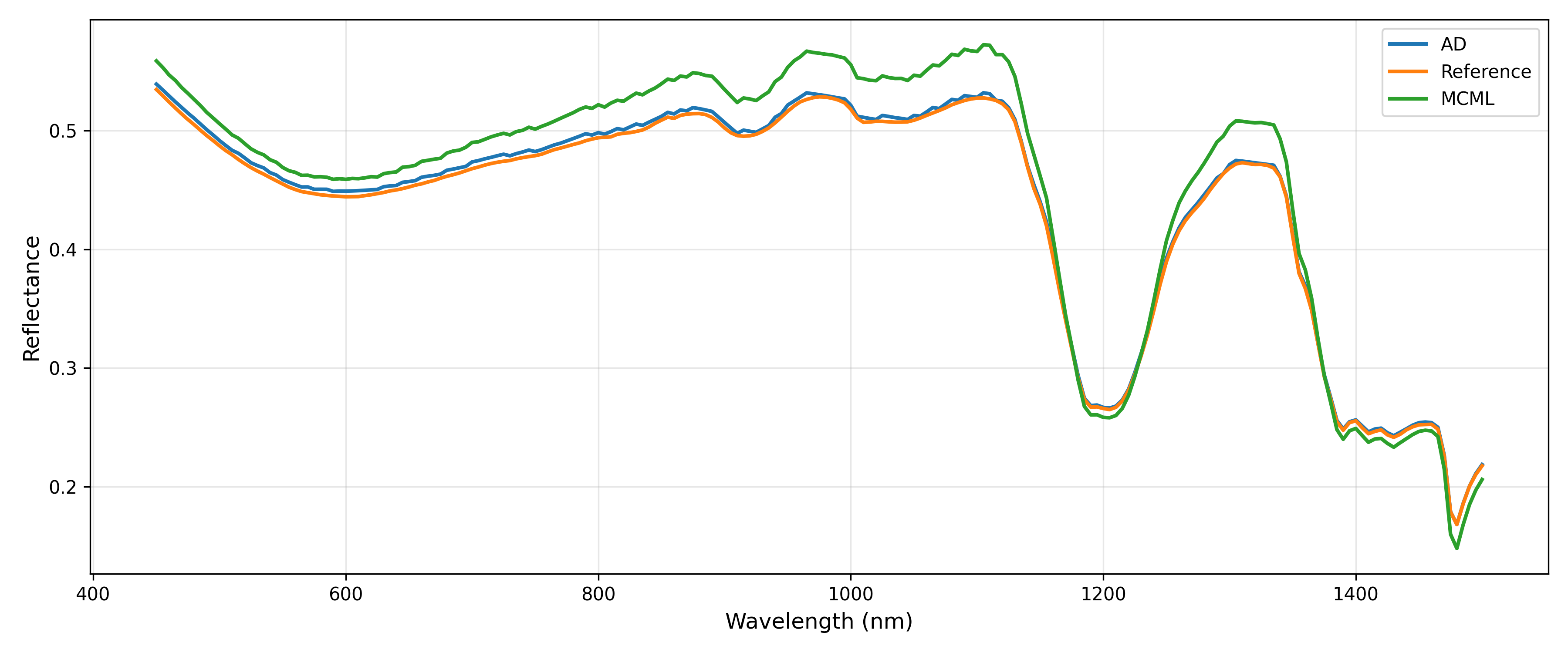
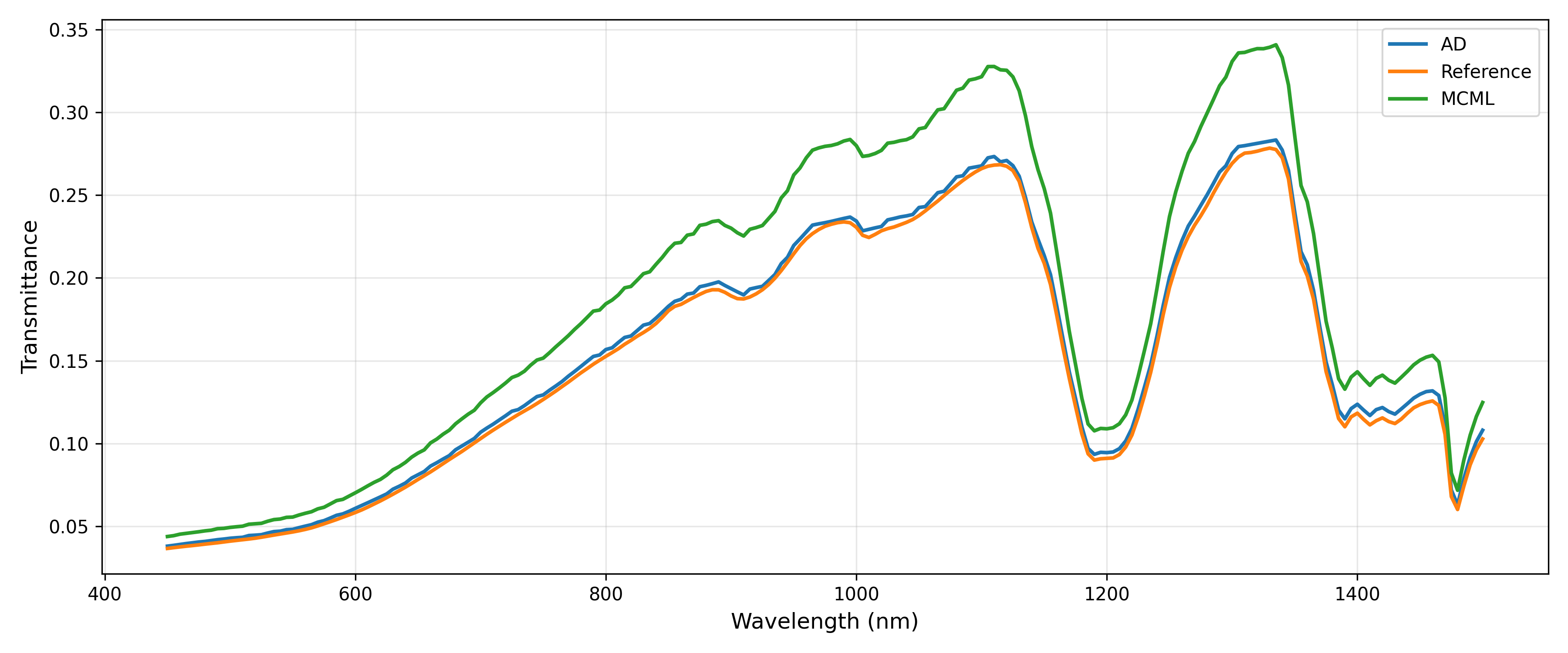
The forward simulation results show excellent agreement between MOP-MCML and AD simulations with factory $R$/$T$ data, validating the accuracy of our forward simulation tools. It’s worth noting that theoretically $R + T < 1$ due to internal absorption losses. As thickness increases, Transmittance $T$ decreases monotonically while Reflectance $R$ remains relatively constant, consistent with the Beer-Lambert law.
3. Experimental Measurement
3.1 Measurement System
We employed a dual-band spectrometer system from Avantes, covering visible to near-infrared wavelengths:
- Visible-NIR Band: 400–1100 nm
- Near-Infrared Band: 900–2500 nm
The two bands overlap in the 900–1100 nm region to ensure spectral continuity.
3.2 Dual Integrating Sphere Measurement Principle
The dual integrating sphere method is a standard technique for measuring diffuse reflectance and transmittance, offering the following advantages:
- Collects all scattered light from the sample, independent of angular distribution
- Eliminates the influence of specular reflection
- Conforms to the diffuse boundary conditions assumed by IAD and AD models
3.2.1 Reflectance Measurement
Configuration parameters:
- 400–1100 nm detector: Integration time 3 ms, averaging 10 times
- 900–2500 nm detector: Integration time 10 ms, averaging 10 times
Measurement procedure:
- Block the beam and acquire dark background (DARK)
- Use PTFE standard white reference, defining $R_{\text{ref}} = 100%$
- Mount the Phantom between dual integrating spheres and measure reflection spectrum $R_{\text{meas}}$
3.2.2 Transmittance Measurement
Configuration parameters:
- 400–1100 nm detector: Integration time 20 ms, averaging 10 times
- 900–2500 nm detector: Integration time 50 ms, averaging 10 times
Measurement procedure:
- Block the beam and acquire dark background (DARK)
- Remove the sample, open the port, defining $T_{\text{ref}} = 100%$
- Mount the Phantom between dual integrating spheres and measure transmission spectrum $T_{\text{meas}}$
3.3 Data Preprocessing
Due to different resolutions and characteristics of the two-band spectrometers, data preprocessing is necessary:
- Band Stitching: Smooth transition in the 900–1100 nm overlap region
- Resampling: Resample from original sampling intervals to 1 nm intervals, covering 450–2000 nm band
- Smoothing: Apply Savitzky-Golay filter (window length 21, polynomial order 3) to reduce noise
After processing, we obtained $R$/$T$ spectral data covering 450–2000 nm band at 1 nm intervals.
4. Measurement Data Correction Method
4.1 Necessity of Correction Analysis
Comparing measurement data with factory standard data revealed:
- Reflectance $R$: Measured values significantly exceed factory standard values (approximately 40% deviation), though waveform trends are consistent
- Transmittance $T$: Values are relatively close but still exhibit systematic deviation
After communication with QUELimaging technical support, deviations were attributed to:
- Measurement equipment differences (different spectrophotometers)
- Measurement principle differences (different calibration standards)
- Light source and detector characteristic differences
Therefore, establishing systematic correction functions to map measurement data to the factory standard coordinate system became necessary.
4.2 Normalized Trend Mapping Method
4.2.1 Basic Principle
We assume a nonlinear mapping relationship exists between measurement data $R_{\text{meas}}$ and factory standard $R_{\text{fac}}$. We adopted a segmented strategy:
- 450–1500 nm band: Factory data available as reference, enabling direct learning of the mapping relationship
- 1500–2000 nm band: No factory data available, requiring extrapolation based on measured trends
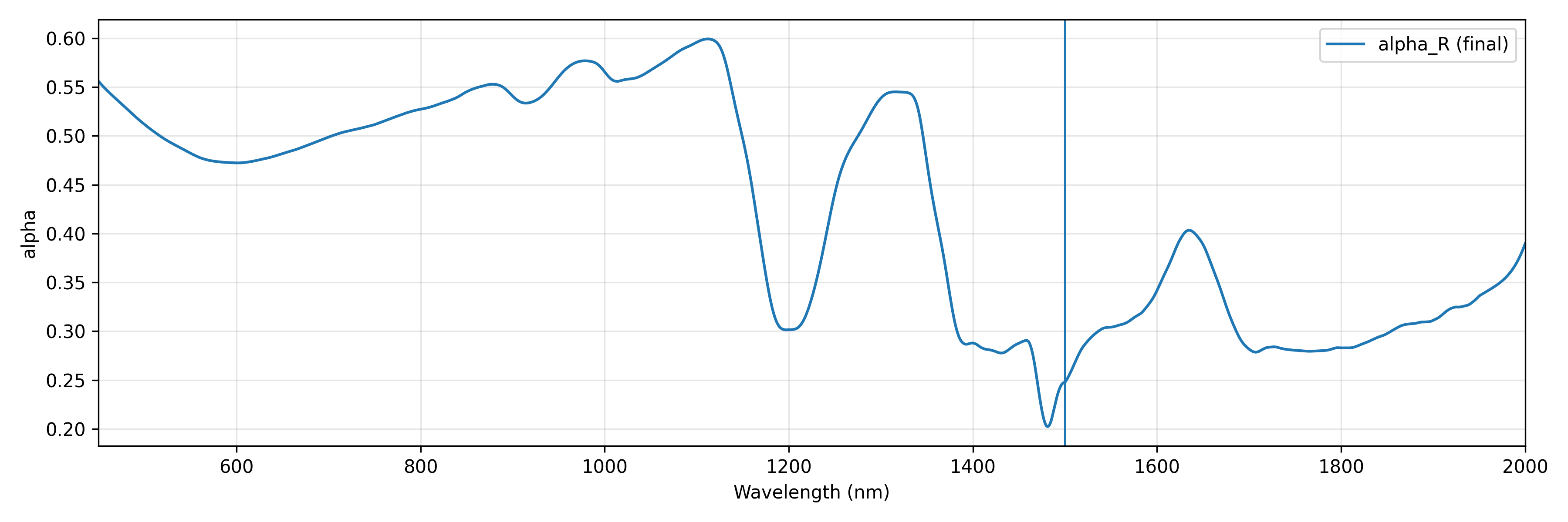
4.2.2 Reflectance Correction Function $\alpha(\lambda)$
For reflectance, due to its low sensitivity to sample thickness, we jointly utilize data from three thicknesses ($i \in {3, 4, 5}$ mm) to construct a unified correction function $\alpha(\lambda)$. For each wavelength $\lambda$, we solve via multi-thickness least-squares optimization:
$$
\alpha(\lambda) = \arg\min_{\alpha} \sum_{i} \left( \alpha \cdot R^{\mathrm{meas}}_i(\lambda) - R^{\mathrm{std}}_i(\lambda) \right)^2
$$
where $R^{\mathrm{meas}}_i(\lambda)$ represents measured reflectance and $R^{\mathrm{std}}_i(\lambda)$ represents factory standard reflectance. Multi-thickness joint optimization enhances $\alpha(\lambda)$ robustness and reduces the influence of single-thickness measurement noise. The corrected reflectance is:
$$
R^{\mathrm{corr}}_i(\lambda) = \alpha(\lambda) \cdot R^{\mathrm{meas}}_i(\lambda)
$$
Learning Phase (450–1500 nm):
- Apply min-max normalization to measurement and factory data:
$$
R_n = \frac{R - R_{\min}}{R_{\max} - R_{\min}}
$$
-
Establish mapping $M: R_{n,\text{meas}} \to R_{n,\text{fac}}$ in normalized space:
- Merge all $(R_{n,\text{meas}}, R_{n,\text{fac}})$ point pairs from three thicknesses
- Obtain discrete $(R_{n,\text{meas}}, R_{n,\text{fac}})$ point pairs using binning statistics
- Construct smooth mapping using PCHIP (Piecewise Cubic Hermite Interpolating Polynomial) interpolation
-
For each wavelength $\lambda$ and each thickness $i$, generate target value $R^{\text{target}}_i(\lambda)$ through normalized mapping, then solve $\alpha(\lambda)$ via least-squares optimization:
$$
\alpha(\lambda) = \arg\min_{\alpha} \sum_{i} \left( \alpha \cdot R^{\text{meas}}_i(\lambda) - R^{\text{target}}_i(\lambda) \right)^2
$$
- Apply Savitzky-Golay smoothing (window 31, polynomial 3)
Extrapolation Phase (1500–2000 nm):
-
Using the learned normalized mapping $M$, generate target values for 1500–2000 nm measurement data by applying the same normalization transform learned in the 450–1500 nm range
-
Calculate $\alpha_{\text{ext}}(\lambda)$ for the extrapolation region and apply strong smoothing (window 101, polynomial 3)
-
Use smoothstep function for smooth stitching in 1480–1520 nm transition region, creating a weighted blend between the learned correction $\alpha_{\text{learn}}(\lambda)$ and extrapolated correction $\alpha_{\text{ext}}(\lambda)$ to ensure continuity
-
Endpoint Constraint: Add decay factor in 1900–2000 nm region, ensuring $R(2000,\text{nm}) < 0.35$
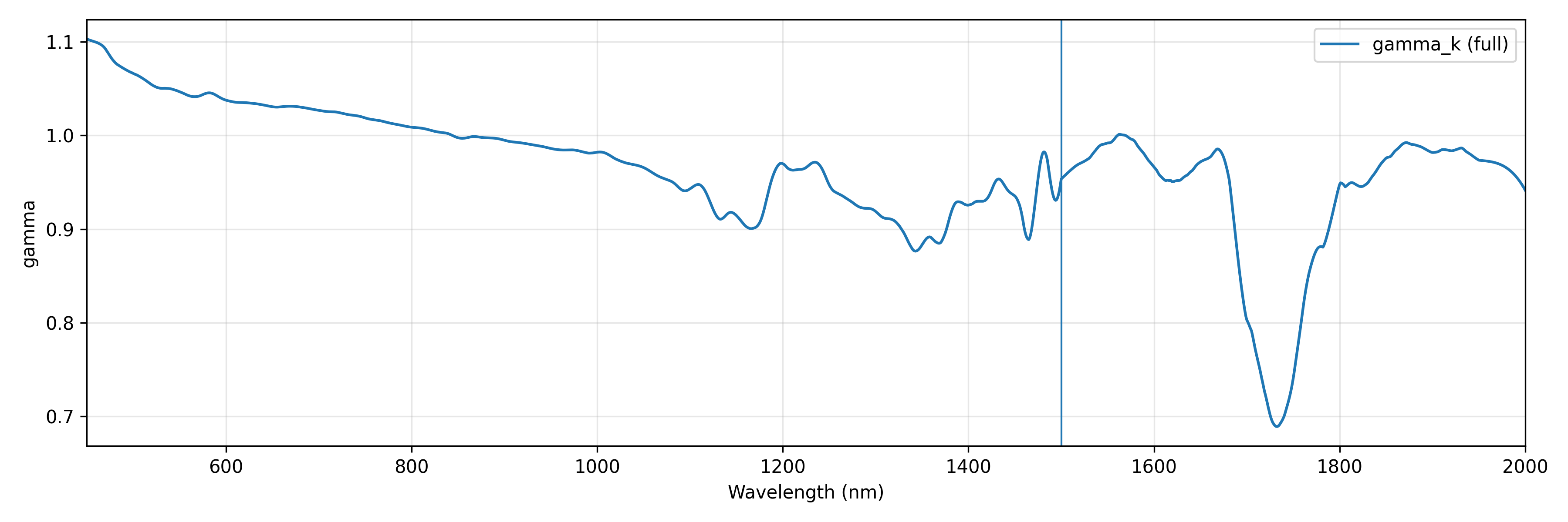
4.2.3 Transmittance Correction Function $\gamma(\lambda)$
Transmittance correction is performed in the absorption coefficient domain based on the Beer-Lambert law:
$$
T = \exp(-k \cdot d)
$$
where $k$ is the effective attenuation coefficient and $d$ is thickness. Since transmittance is sensitive to thickness, we similarly utilize data from three thicknesses ($i \in {3, 4, 5}$ mm) jointly to construct correction function $\gamma(\lambda)$. In $k$-space, we solve via multi-thickness least-squares optimization:
$$
\gamma(\lambda) = \arg\min_{\gamma} \sum_{i} \left( \gamma \cdot k^{\text{meas}}_i(\lambda) - k^{\text{std}}_i(\lambda) \right)^2
$$
where $k^{\text{meas}}_i(\lambda) = -\ln(T^{\text{meas}}_i(\lambda))/d_i$ is the effective attenuation coefficient from measurement data, and $k^{\text{std}}_i(\lambda) = -\ln(T^{\text{std}}_i(\lambda))/d_i$ is from factory standard. The corrected transmittance is:
$$
T^{\text{corr}}_i(\lambda) = \exp\left(-\gamma(\lambda) \cdot k^{\text{meas}}_i(\lambda) \cdot d_i\right)
$$
We employ the same normalized trend mapping method as for reflectance:
- 450–1500 nm learning phase: Joint optimization across three thicknesses in $k$-space to obtain $\gamma(\lambda)$
- 1500–2000 nm extrapolation phase: Generate targets based on normalized trend mapping of $T$, calculate $\gamma_{\text{ext}}(\lambda)$ in $k$-space
- Transition region stitching: Use smoothstep for smooth transition at 1480–1520 nm
- Envelope constraint: Clip $T_{\text{corr}}$ to factory data envelope range in 450–1500 nm
4.3 Correction Results
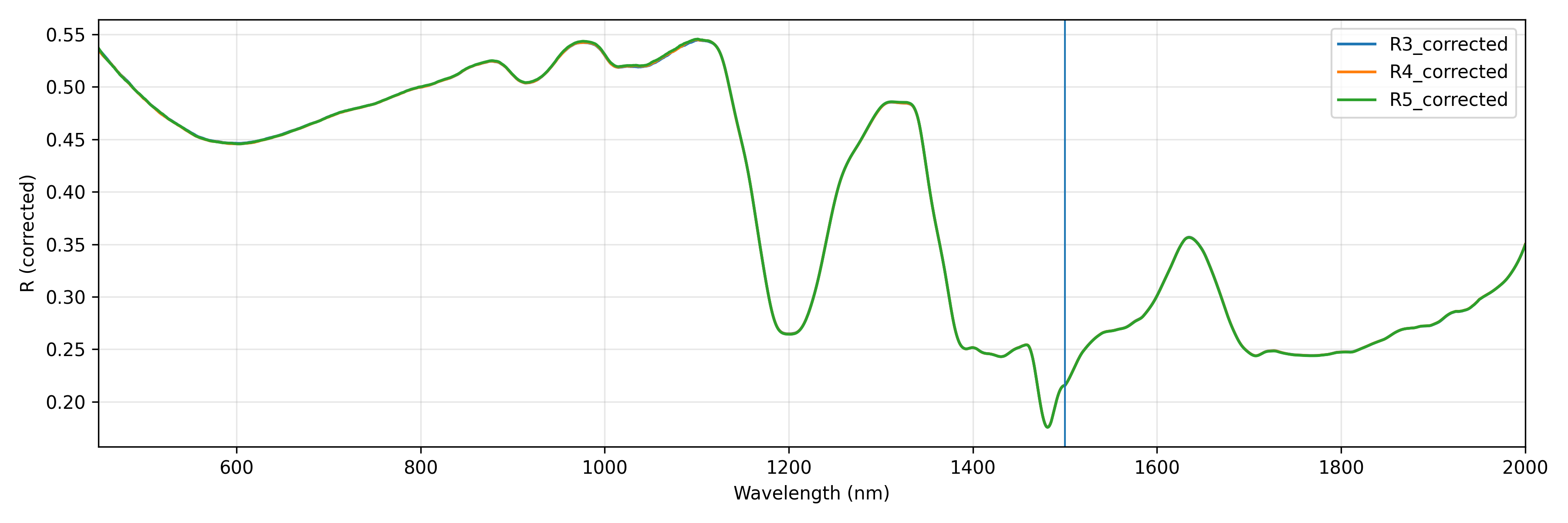
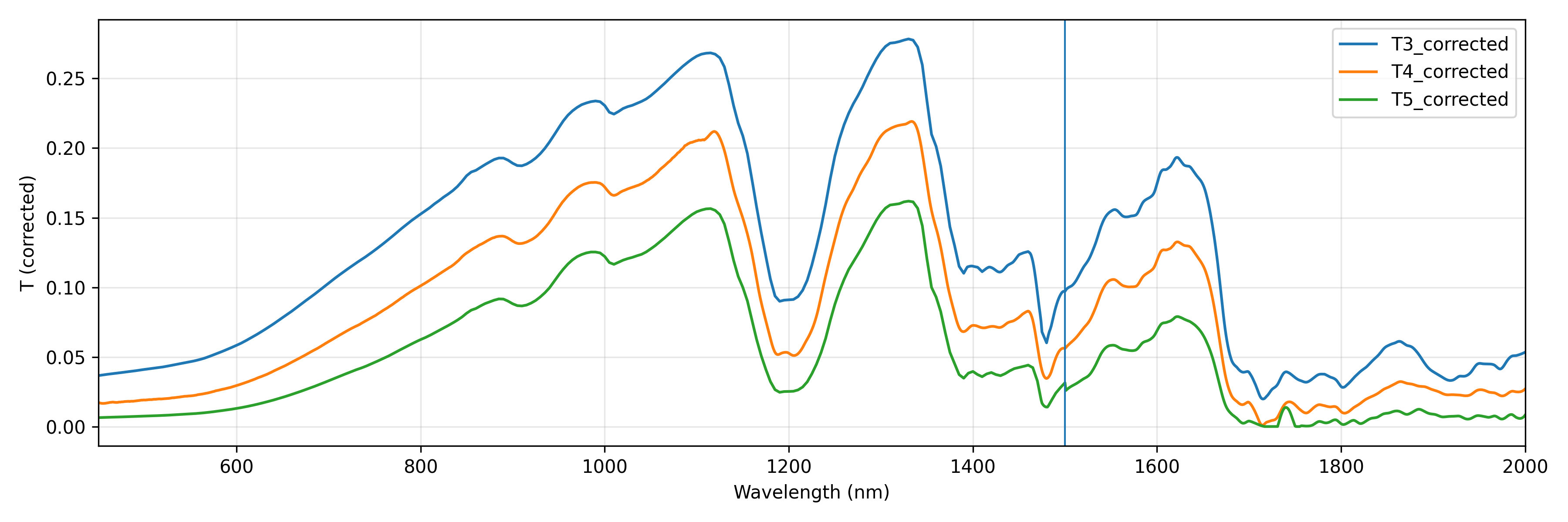
The corrected $R$/$T$ data show excellent agreement with factory standards in the 450–1500 nm band. Extrapolation results for the 1500–2000 nm band conform to physical trends (slight decrease in reflectance, continued decrease in transmittance).
5. Closed-Loop Validation
5.1 IAD Inversion Validation
We inverted the corrected $R$/$T$ data (450–2000 nm) through IAD to obtain optical parameters $\mu_a$ and $\mu_s’$, comparing them against factory standard parameters:
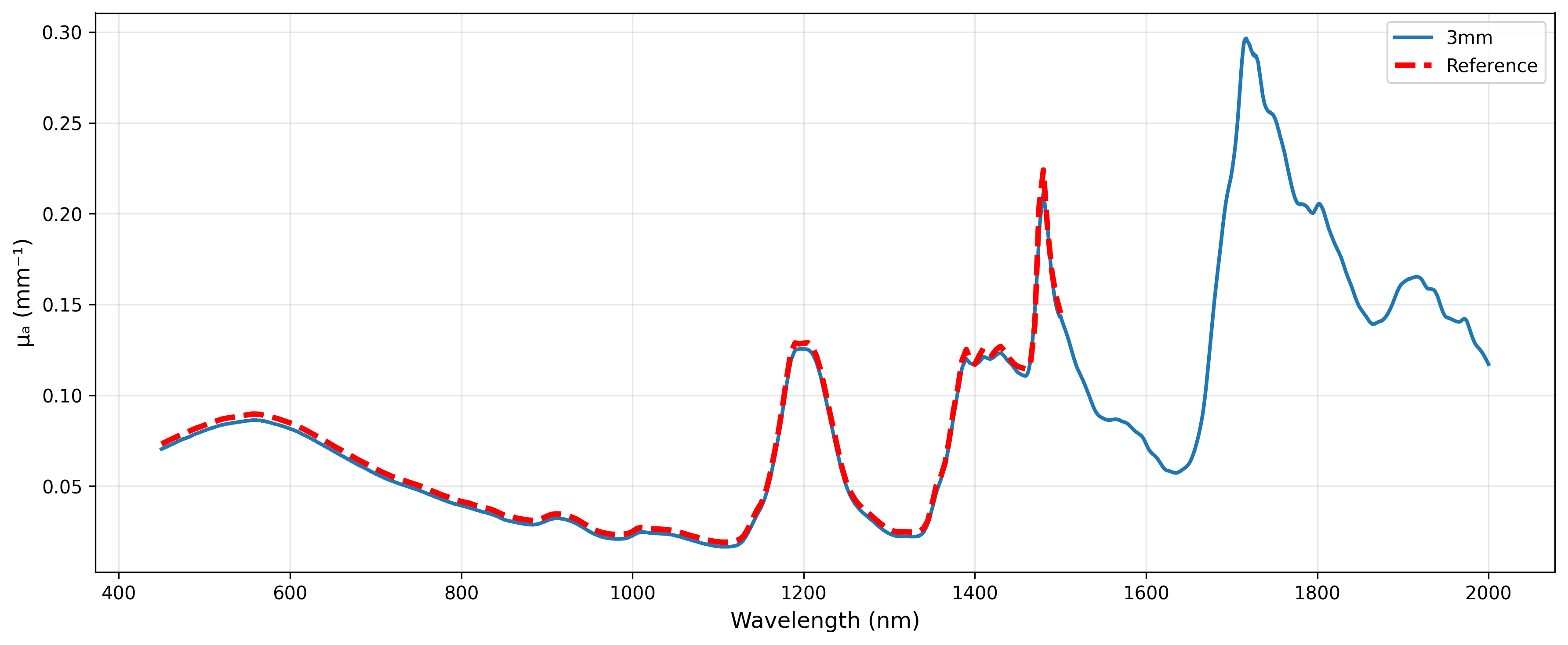
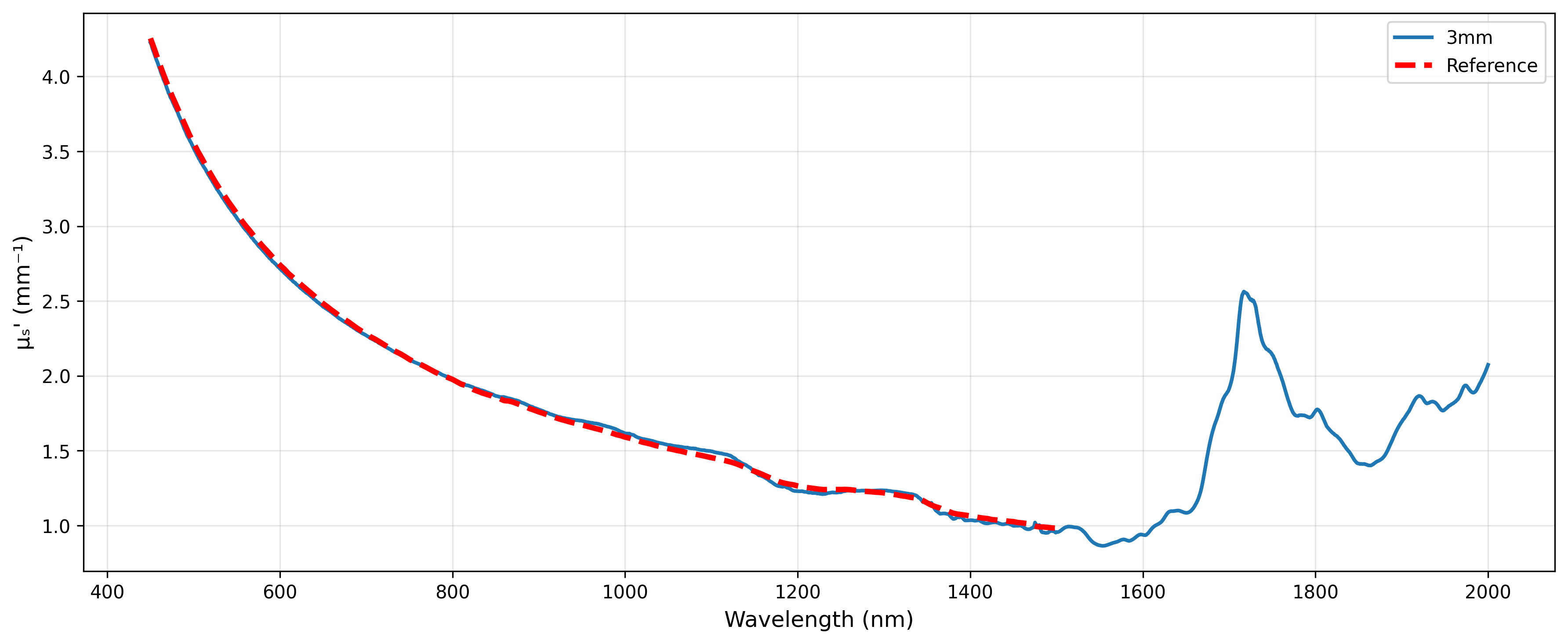
The inversion results demonstrate that optical parameters retrieved from corrected data show high consistency with factory standards in the 450–1500 nm band, validating the effectiveness of our correction method. Although no factory reference data exists for the 1500–2000 nm band, the inverted curves remain smooth and continuous without non-physical discontinuities, indicating reasonable extrapolation correction.
5.2 Forward Simulation Validation
Using optical parameters inverted from the full band (450–2000 nm) via IAD, we performed forward simulations through MOP-MCML and AD to calculate $R$/$T$:
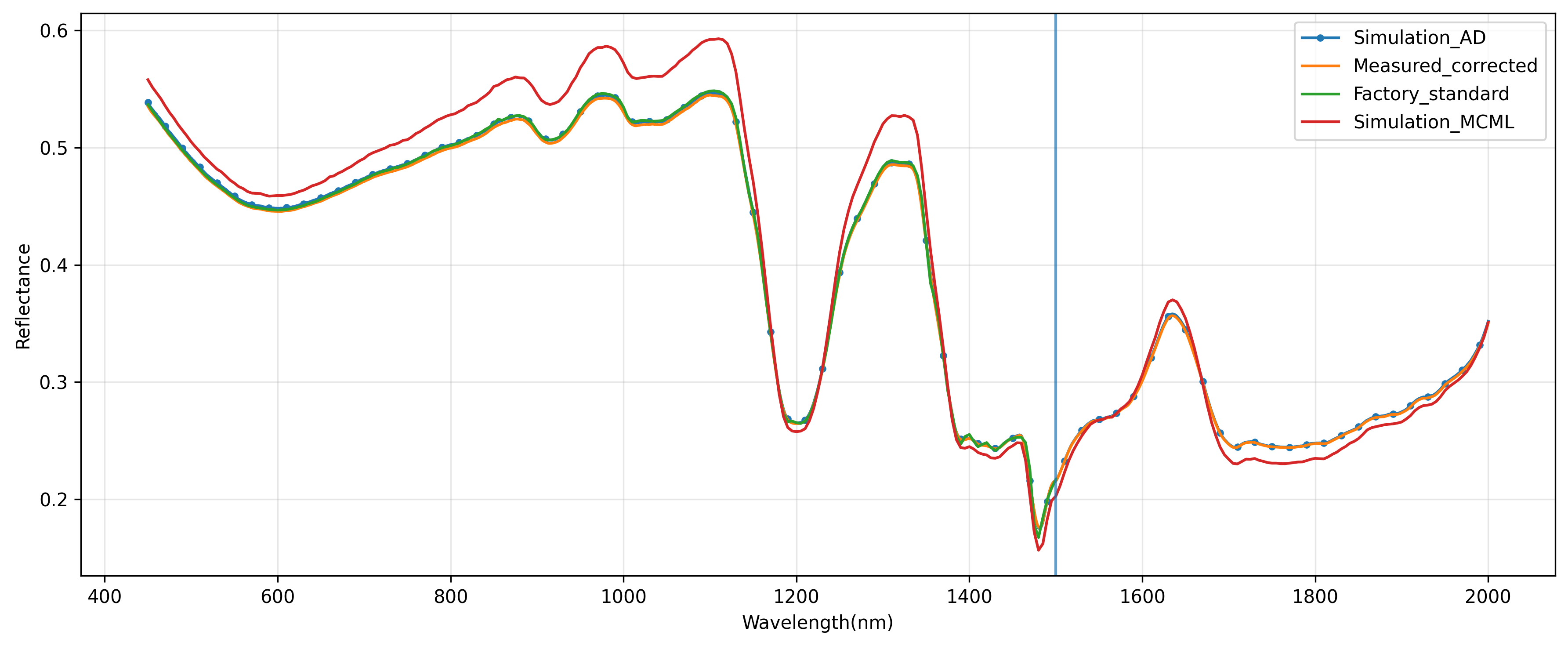
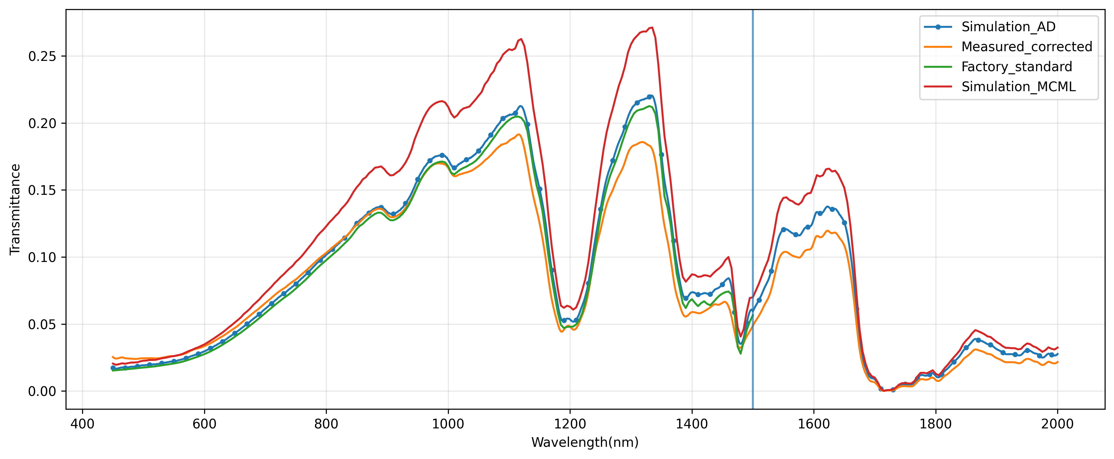
Forward simulation results reveal:
- MOP-MCML and AD simulations: Highly consistent results from both simulation tools, mutually validating each other
- Comparison with corrected measurements: Forward simulation results agree well with corrected measurement data
- Comparison with factory standards: In the 450–1500 nm overlap region, forward results are fundamentally consistent with factory standards
At this point, we have completed a full validation loop:
Factory data validation loop:
$$
R/T_{\text{fac}} \xrightarrow{\text{IAD}} \mu_a, \mu_s’ \xrightarrow{\text{MCML/AD}} R/T \approx R/T_{\text{fac}}
$$
Measurement data validation loop:
$$
R/T_{\text{meas}} \xrightarrow{\alpha, \gamma} R/T_{\text{corr}} \xrightarrow{\text{IAD}} \mu_a, \mu_s’ \xrightarrow{\text{MCML/AD}} R/T \approx R/T_{\text{corr}}
$$
6. Discussion
6.1 Advantages of the Normalized Trend Mapping Method
Traditional linear correction methods (e.g., $R_{\text{corr}} = \alpha_0 \cdot R_{\text{meas}}$) assume constant correction coefficients and cannot handle wavelength-dependent systematic deviations. Our proposed dynamic normalized mapping method offers the following advantages:
- Nonlinear Mapping: Captures nonlinear relationships through PCHIP interpolation, adapting to complex instrument response functions
- Multi-Thickness Joint Optimization: Simultaneously leverages data from three thicknesses, improving correction function robustness
- Smooth Extrapolation: In bands without reference data, performs reasonable extrapolation based on learned trends, avoiding non-physical discontinuities
- Physical Constraints: Ensures correction results comply with physical laws through endpoint constraints and envelope clipping
6.2 Uncertainty in the 1500–2000 nm Band
Since factory data only covers 450–1500 nm, correction for the 1500–2000 nm band relies on extrapolation and carries certain uncertainty. However, we mitigated risks through the following methods:
- Smooth Extrapolation: Using larger smoothing windows (101) reduces the influence of high-frequency noise
- Envelope Constraints: Endpoint constraints ensure $R(2000)$ does not exceed reasonable upper limits
- Closed-Loop Validation: Extrapolation results underwent bidirectional verification through IAD inversion and MOP-MCML forward simulation, showing no non-physical behavior
6.3 Accuracy of Simulation Tools
The highly consistent results from MOP-MCML and AD forward simulation tools, along with their excellent agreement with factory standards, validate the reliability of Monte Carlo and Adding-Doubling methods in biological tissue optical simulation. For other wavelength ranges and optical parameters, these tools can serve as trustworthy simulation benchmarks.
7. Conclusion
Through systematic experimental and data processing procedures, this study achieved bidirectional verification between simulation and measurement based on Phantom F04:
- Factory Data Verification: Validated the internal consistency of factory-provided data and the accuracy of simulation tools through IAD inversion and MOP-MCML/AD forward simulation
- Normalized Trend Mapping Correction: Proposed a nonlinear correction method based on normalized space, successfully establishing the mapping relationship between measurement data and factory standards
- Full-Band Extrapolation: For the 1500–2000 nm band without factory reference, performed reasonable extrapolation based on learned trends, with results verified as reasonable through closed-loop validation
- Complete Closed-Loop Verification: Established dual verification loops: “Factory data → IAD inversion → Forward simulation → Factory data” and “Measurement data → Correction → Inversion → Forward simulation → Corrected data”
This study validates the accuracy and reliability of simulation tools like MOP-MCML and IAD in biological tissue optical modeling, providing a solid experimental foundation for subsequent simulation research based on these tools. The normalized trend mapping method can be generalized to other optical measurement data correction scenarios requiring cross-instrument and cross-standard alignment.
References
- MOP-MCML User Guide: https://www.wenzheng.eu/2025/09/09/MOP_MCML/
- IAD Algorithm Original Paper: Scott Prahl, “The Adding-Doubling Method,” Applied Optics, 32:559-568 (1993)
- QUELimaging Phantom F04: https://shop.quelimaging.com/product/tissue-equivalent-optical-phantoms/